

In part 1 of this column on the basics of the Ethernet protocol, I noted that since Ethernet is so pervasive in local area networks (LANs), understanding the nuts and bolts of Ethernet function will pay off for the HTM service professional. As explained in part 1, Ethernet lies low on the OSI model, implying that Ethernet must perform its duties before any other network communication can happen.
Part 1 focused on the Ethernet protocol that merges packet data into network traffic to send it on its way, delivering the network LAN communication. A key concept was that each node on the network is responsible for its own communication, transmitting data packets into the ongoing LAN traffic. In other words, there is no communication master regulating overall network traffic. Each node arbitrates for LAN access when it needs to transmit.
In this second and last installment on this topic, we will examine the Ethernet packet structure to show how the Ethernet recipient portion of the protocol operates.
Ethernet Packet Structure
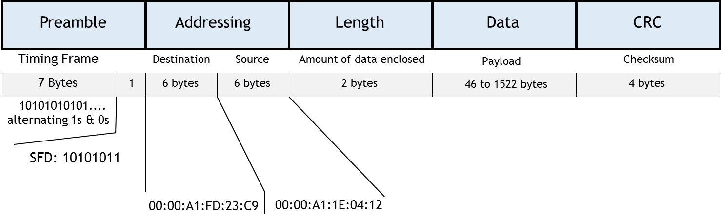
Figure 1. The Ethernet packet architecture. Click to enlarge.
Figure 1 shows the Ethernet data packet architecture. Recall that the nodes use the Carrier Sense Multiple Access with Collision Detection (CSMS/CD) protocol flowchart to merge into network traffic.
The beginning of the packet is a timing frame, which is part of the preamble. The timing frame is 7 bytes, or 56 bits, of alternating 1’s and 0’s. Because Ethernet uses asynchronous serial communication, there is no separate clock signal. The clock is modulated into the data using a type of Manchester Encoding. Manchester encoding ensures that each bit period is divided into two complementary halves. A negative to positive voltage change at this halfway mark represents sending a digital 1; a positive to negative change at halfway represents a digital zero. In this way, the recipient can recover the embedded clock signal to sync the transmission.
The idea of the timing frame is to help the receiver’s clock get in sync with the incoming data packet, in order to successfully recover the 1’s and 0’s of the communication. At the end of the preamble is the start frame delimiter (SFD). The SFD is 8 bits in length of alternating 1’s and 0’s ending with “1 1.” The “1 1” indicates to the recipient that the next series of bits is the packet information. The first part of the packet information is the Ethernet addressing. The destination address comes first, identifying the recipient node this packet is intended for. The second address is the source address, indicating who sent it.
The Ethernet Address
Ethernet addresses consist of 6 bytes of information. Each byte is written in hexadecimal format and is delimited by a colon. Looking at the examples shown in figure 1, 00:00:A1:FD:23:C9 is the destination address of the intended recipient. Next the Ethernet packet architecture indicates the sender or source address—in this case, 00:00:A1:1E:04:12—which is, obviously, different from the destination address.
Following the addressing segment of the packet is a two-byte field specifying how much data the packet is carrying. The data payload can range from 46 to 1522 bytes in length—not a lot of space for data. There are other higher layer protocols that break large files into pieces where each piece is sized for the Ethernet envelope.
Finally, at the end of the packet there is a 4-byte checksum called the cyclic redundancy check (CRC). The CRC adds up all the 1’s and 0’s of the packet fields, 4-bytes wide, or 4 bytes at a time, and comes up with a 4-byte value or sum to place in this last field.
The Receiving Side
To receive a data packet, the Ethernet circuitry first syncs data clocks with the incoming timing frame. Next, if the recipient recognizes the destination address as “my address” (called a unicast address), the recipient—let’s call it Node A—will run a checksum on the packet to compare with the checksum value sent. That will tell Node A if the packet and data arrived intact. If the packet somehow got corrupted, the checksums won’t match and Node A simply throws the packet away into the proverbial bit bucket. In other words, there is no way for Node A to discern where in the packet the corruption occurred. Node A is not going to spend any time in trying to figure it out at this level. Some network protocol higher in the OSI model worries about full packet data recovery—not a concern at this stage.
If the packet does not contain Node A’s unicast address, it will just be thrown away. In other words, if it’s not for Node A, Node A don’t care. (Note that there is also something called a broadcast address—a packet meant to all nodes to read, such as a public network announcement of some kind. Broadcast addresses are all digital 1’s or in hexadecimal would be FF:FF:FF:FF:FF:FF.)
If the data packet has Node A’s unicast address as the destination, and if the checksums match, Node A will accept the packet. If it is addressed to Node A, the node can check the source address to see who sent it. Then it will check to see how much data there is in the payload, so as to be able extract the payload data to forward it upstream to the higher layers in the OSI model. A broadcast packet is treated the same way as a unicast addressed packet: If the checksum analysis checks out, Ethernet extracts the payload and passes it upstream.
Slot Time
While we’re examining the Ethernet packet, let’s take a moment to talk about slot time. Slot time is the minimum amount of time a data packet will occupy the media or wire. Let’s start with the minimum payload or smallest data packet at 46 bytes.
Adding 46 to the checksum, which is 4 bytes, equals 50 bytes. Adding 12 bytes of addressing, 6 bytes for each address, adds up to 62 bytes. Finally, adding the 2-byte data-length field, we get to a grand total of 64 bytes for the shortest Ethernet data packet. Converted to bits, 64 bytes multiplied by 8 equals 512 bits.
At a network speed of 10 MBits, this means that each bit width is 0.1 µsecond. Multiplying 0.1 µS times 512 bits comes to 51.2 µS. The shortest Ethernet packet will occupy the line for 51.2 µS. Does that number sound familiar? It’s what the Ethernet protocol uses as a constant in its back-off scheme, as we saw in part 1. Each node needs to wait at least the amount of time that the shortest data packet would occupy the wire before it attempts to merge into traffic again.
Faster Ethernet Effects on Slot Time
If this network was running at 100 Megabits per second, the slot time would scale accordingly and the wait time factor would be 5.12 µS. Everything else—the data packet structure and the CSMA/CD scheme—remains the same.
If this were a Gigabit network, it would add to or pad the data payload with extra zeroes to give all the nodes a chance to sense voltages on the cable. Due to its speed, the Gigabit Ethernet uses about 4000 bits as the smallest data packet. In other words, it scales the same way but adds a fudge factor and waits for approximately 4 µS as the slot time.
Regardless, the idea remains the same: We wait for an amount of time representing the shortest or smallest data packet.
When we speak of serial communications here, we’re usually talking about 10BASE-T, which is Ethernet’s common cabling. There is also 10BASE-F, which is fiber optics cabling. Fiber optics can be up to a kilometer in each segment length, but still consists of a point-to-point connection, like a twisted pair. If I want to connect across town, I can use a couple of repeaters, and a couple of kilometers of fiber optic cable. A kilometer, of course, is approximately six-tenths of a mile—now we’re getting somewhere! Fiber also supports much faster speeds.
Conclusion
Ethernet fundamentals boil down to the CSMS/CD process to transmit data (the process shown in the flow chart in part 1 of this series). It entails some checks and balances when receiving an Ethernet packet, such as syncing clocks, checking addressing, and performing a quality check to complete the data transfer. Recall that Ethernet resides at layer 2, the Data Link layer of the OSI model, and that the layer consists of media access control (MAC) and logical link control (LLC) sub layers. With this in mind, think of the flow chart process as the LLC or software portion, and of the packet as the MAC layer or hardware portion. This is also why Ethernet addresses are known as MAC addresses.
Ethernet functionality has essentially remained the same for a long time because it works. It has stood the test of time. Will some kind of new technology come along that is faster, cheaper, and denser electronically enough to ultimately affect the fundamentals of Ethernet communication? Probably. But it darn sure ought to be backward compatible!
Jeff Kabachinski is the director of technical development for Aramark Healthcare Technologies in Charlotte, NC. For more information, contact editorial director John Bethune at [email protected].
Lead photo copyright © Davizro | Dreamstime.com